Parkinson’s Disease Progression Modeling with Leaspy

This example demonstrates how to use Leaspy to model the progression of Parkinson’s disease using synthetic data.

The following imports bring in the required modules and load the synthetic dataset from Leaspy. The dataset contains repeated measurements for multiple subjects over time.

from leaspy.datasets import load_dataset
from leaspy.io.data import Data

df = load_dataset("parkinson")

The first few rows of the dataset provide an overview of its structure.

df.head()

		MDS1_total	MDS2_total	MDS3_off_total	SCOPA_total	MOCA_total	REM_total	PUTAMEN_R	PUTAMEN_L	CAUDATE_R	CAUDATE_L
ID	TIME
GS-001	71.354607	0.112301	0.122472	0.171078	0.160001	0.275257	0.492485	0.780210	0.676774	0.622611	0.494641
	71.554604	0.140880	0.109504	0.118693	0.135852	0.380934	0.577203	0.751444	0.719796	0.618434	0.530978
	72.054604	0.225499	0.270502	0.061310	0.211134	0.351172	0.835828	0.823315	0.691504	0.717099	0.576978
	73.054604	0.132519	0.253548	0.258786	0.245323	0.377842	0.566496	0.813593	0.787914	0.770048	0.709486
	73.554604	0.278923	0.321920	0.143350	0.223102	0.292768	0.741811	0.888792	0.852720	0.797368	0.715465

The total number of unique subjects present in the dataset is shown below.

n_subjects = df.index.get_level_values("ID").unique().shape[0]
print(f"{n_subjects} subjects in the dataset.")

200 subjects in the dataset.

The dataset is separated into a training set and a test set. The first portion of the data is used for training and the remaining portion for testing.

df_train = df.loc[:"GS-160"][["MDS1_total", "MDS2_total", "MDS3_off_total"]]
df_test = df.loc["GS-161":][["MDS1_total", "MDS2_total", "MDS3_off_total"]]

The pandas DataFrames are converted to Leaspy Data objects for further modeling.

data_train = Data.from_dataframe(df_train)
data_test = Data.from_dataframe(df_test)

The logistic model is imported and initialized. A two-dimensional source space is chosen to represent disease progression trajectories.

from leaspy.models import LogisticModel

model = LogisticModel(name="test-model", source_dimension=2)

Visualization utilities from Leaspy and Matplotlib are imported.

import matplotlib.pyplot as plt
from leaspy.io.logs.visualization.plotting import Plotting

leaspy_plotting = Plotting(model)

/home/docs/checkouts/readthedocs.org/user_builds/leaspy/checkouts/472/src/leaspy/io/logs/visualization/plotting.py:42: FutureWarning: Plotting will soon be removed from Leaspy, please use Plotter instead.
  warnings.warn(

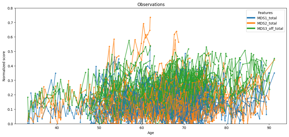
Data that will be used to fit the model can be illustrated as follows:

ax = leaspy_plotting.patient_observations(data_train, alpha=0.7, figsize=(14, 6))
ax.set_ylim(0, 0.8)  # The y-axis is adjusted for better visibility.
plt.show()

The model is fitted to the training data using the MCMC-SAEM algorithm. A fixed seed is used for reproducibility and 100 iterations are performed.

model.fit(
    data_train,
    "mcmc_saem",
    seed=0,
    n_iter=100,
    progress_bar=False,
)

Fit with `AlgorithmName.FIT_MCMC_SAEM` took: 1.75s

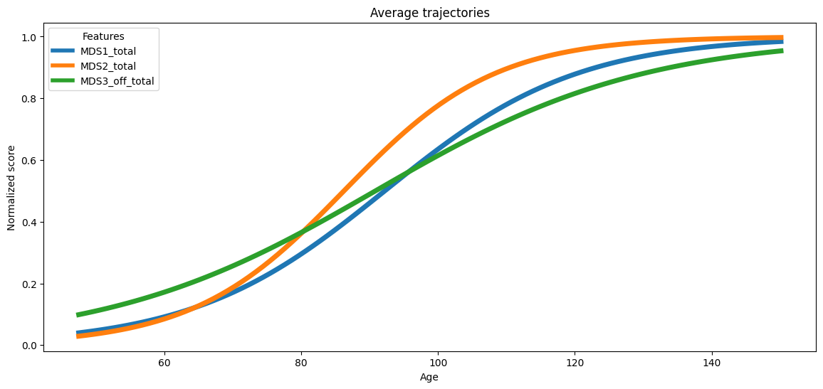
The average trajectory estimated by the model is displayed. This figure shows the mean disease progression curves for all features.

ax = leaspy_plotting.average_trajectory(
    alpha=1, figsize=(14, 6), n_std_left=2, n_std_right=8
)
plt.show()

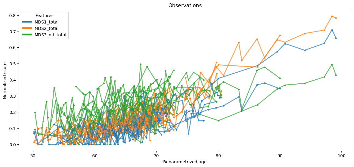
Individual parameters are obtained for the test data using the personalization step.

ip = model.personalize(data_test, "scipy_minimize", seed=0, progress_bar=False, use_jacobian=False)

Personalize with `AlgorithmName.PERSONALIZE_SCIPY_MINIMIZE` took: 7.41s

The test data with individually re-parametrized ages is plotted below.

ax = leaspy_plotting.patient_observations_reparametrized(
    data_test, ip, alpha=0.7, linestyle="-", figsize=(14, 6)
)
plt.show()

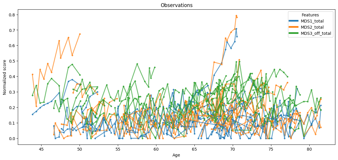
The test data with the true ages (without re-parametrization) is plotted below.

ax = leaspy_plotting.patient_observations(
    data_test,
    alpha=0.7,
    linestyle="-",
    figsize=(14, 6),
)
plt.show()

Observations for a specific subject are extracted to demonstrate reconstruction.

import numpy as np

observations = df_test.loc["GS-187"]
print(f"Seen ages: {observations.index.values}")
print("Individual Parameters : ", ip["GS-187"])

timepoints = np.linspace(60, 100, 100)
reconstruction = model.estimate({"GS-187": timepoints}, ip)

Seen ages: [61.34811783 62.34811783 63.84811783 64.34812164 67.84812164 68.34812164
 69.34812164 69.84812164 70.84812164 71.34812164 71.84812164 72.34812164
 72.84812164 73.34812164]
Individual Parameters :  {'sources': [1.3116443157196045, 0.7219943404197693], 'tau': [73.46703338623047], 'xi': [0.06865404546260834]}

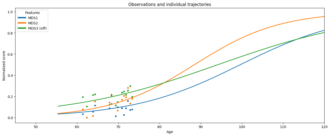
The reconstructed trajectory along with the actual observations for selected subjects is displayed.

ax = leaspy_plotting.patient_trajectories(
    data_test,
    ip,
    patients_idx=["GS-187"],
    labels=["MDS1", "MDS2", "MDS3 (off)"],
    figsize=(16, 6),
    factor_future=5,
)
ax.set_xlim(45, 120)
plt.show()

This concludes the Parkinson’s disease progression modeling example using Leaspy. Leaspy is also capable of handling various other types of models, as the Joint Models, which will be explored in the next section.