Mixture Model

This notebook contains the code for a simple implementation of the Leaspy Mixture model on synthetic data. Before implementing the model take a look at the relevant mathematical framework in the user guide.

The following imports are required libraries for numerical computation, data manipulation, and visualization.

import os
import matplotlib.pyplot as plt
import numpy as np
import pandas as pd
import torch
import leaspy
from leaspy.io.data import Data

This toy example is part of a simulation study, carried out by Sofia Kaisaridi that will be included in an article to be submitted in a biostatistics journal. The dataset contains 1000 individuals each with 6 visits and 6 scores.

leaspy_root = os.path.dirname(leaspy.__file__)
data_path = os.path.join(leaspy_root, "datasets/data/simulated_data_for_mixture.csv")

all_data = pd.read_csv(data_path, sep=";", decimal=",")
all_data["ID"] = all_data["ID"].ffill()
all_data = all_data.set_index(["ID", "TIME"])
all_data.head()

		score_1_normalized	score_2_normalized	score_3_normalized	score_4_normalized	score_5_normalized	score_6_normalized
ID	TIME
subj_1	50.159062	0.197863	0.057787	0.095305	0.141747	0.265511	0.397614
	66.713371	0.418290	0.139975	0.021792	0.119112	0.481825	0.456491
	68.994947	0.397005	0.149633	0.040861	0.128334	0.388164	0.394283
	73.009543	0.330076	0.127369	0.098300	0.348438	0.473187	0.418984
	80.948301	0.530554	0.117444	0.159612	0.339971	0.468804	0.591484

We load the Mixture Model from the leaspy library and transform the dataset in a leaspy-compatible form with the built-in functions.

from leaspy.models import LogisticMultivariateMixtureModel

leaspy_data = Data.from_dataframe(all_data)

Then we fit a model with 3 clusters and 2 sources. Note that we have an extra argument n_clusters than the standard model that has to be specified in order for the mixture model to run.

model = LogisticMultivariateMixtureModel(
    name="multi",
    source_dimension=2,
    dimension=6,
    n_clusters=3,
    obs_models="gaussian-diagonal",
)

model.fit(leaspy_data, "mcmc_saem", seed=1312, n_iter=100, progress_bar=False)
model.summary()

Fit with `AlgorithmName.FIT_MCMC_SAEM` took: 3.96s

================================================================================
                                 Model Summary                                  
================================================================================
Model Name: multi
Model Type: LogisticMultivariateMixtureModel
Features (6): score_1_normalized, score_2_normalized,
    score_3_normalized, score_4_normalized, score_5_normalized,
    score_6_normalized
Sources (2): Source 0 (s0), Source 1 (s1)
Clusters (3): Cluster 0 (c0), Cluster 1 (c1), Cluster 2 (c2)
Observation Models: gaussian-diagonal
Neg. Log-Likelihood: -5265.7297

Training Metadata
--------------------------------------------------------------------------------
Algorithm: AlgorithmName.FIT_MCMC_SAEM
Seed: 1312
Iterations: 100

Data Context
--------------------------------------------------------------------------------
Subjects: 1000
Visits: 6000
Total Observations: 36000

Leaspy Version: 2.0.1
================================================================================

Population Parameters
--------------------------------------------------------------------------------
  betas_mean:
                          s0        s1
            b0       -0.0099    0.0054
            b1       -0.0062    0.0054
            b2        0.0372   -0.0189
            b3        0.0329   -0.0143
            b4        0.0424   -0.0385
                          c0        c1        c2
  probs               0.3247    0.4001    0.2752
  sources_mean:
                          c0        c1        c2
            s0       -1.1791   -0.9338    2.7506
            s1        2.4279   -0.8996   -1.5589
                    score_1.  score_2.  score_3.  score_4.  score_5.  score_6.
  log_g_mean          0.6386    1.6792    2.2111    0.9981    0.4451   -0.0358
                    score_1.  score_2.  score_3.  score_4.  score_5.  score_6.
  log_v0_mean        -5.0169   -5.0958   -6.3110   -5.1638   -5.3070   -5.6924

Individual Parameters
--------------------------------------------------------------------------------
                          c0        c1        c2
  tau_mean           71.0264   66.0683   57.4709
                          c0        c1        c2
  tau_std            10.4716    8.8100   11.6153
                          c0        c1        c2
  xi_mean            -0.1970   -0.2768    0.6348
                          c0        c1        c2
  xi_std              0.8801    0.9058    1.0671

Noise Model
--------------------------------------------------------------------------------
                    score_1.  score_2.  score_3.  score_4.  score_5.  score_6.
  noise_std           0.0744    0.0715    0.0370    0.0625    0.0812    0.0779
================================================================================

First we take a look in the population parameters. With the mixture model we obtain separate values for the tau_mean, xi_mean and the sources_mean for each cluster, as well as the cluster probabilities (probs).

print(model.parameters)

{'betas_mean': tensor([[-0.0099,  0.0054],
        [-0.0062,  0.0054],
        [ 0.0372, -0.0189],
        [ 0.0329, -0.0143],
        [ 0.0424, -0.0385]]), 'log_g_mean': tensor([ 0.6386,  1.6792,  2.2111,  0.9981,  0.4451, -0.0358]), 'log_v0_mean': tensor([-5.0169, -5.0958, -6.3110, -5.1638, -5.3070, -5.6924]), 'noise_std': tensor([0.0744, 0.0715, 0.0370, 0.0625, 0.0812, 0.0779], dtype=torch.float64), 'probs': tensor([0.3247, 0.4001, 0.2752], dtype=torch.float64), 'sources_mean': tensor([[-1.1791, -0.9338,  2.7506],
        [ 2.4279, -0.8996, -1.5589]], dtype=torch.float64), 'tau_mean': tensor([71.0264, 66.0683, 57.4709], dtype=torch.float64), 'tau_std': tensor([10.4716,  8.8100, 11.6153], dtype=torch.float64), 'xi_mean': tensor([-0.1970, -0.2768,  0.6348], dtype=torch.float64), 'xi_std': tensor([0.8801, 0.9058, 1.0671], dtype=torch.float64)}

Then we can also retrieve the individual parameters and the posteriors probabilities of cluster membership. We then consider that the cluster label is the cluster with the biggest probability.

from torch.distributions import Normal

def get_ip(df_leaspy, model):
    """
    leaspy_data : the dataframe with the correct indexing
    leaspy_mixture : the leaspy object after the fit
    """
    ip = pd.DataFrame(df_leaspy.index.get_level_values("ID").unique(), columns=["ID"])

    ip[["tau"]] = model.state["tau"]
    ip[["xi"]] = model.state["xi"]
    ip[["sources_0"]] = model.state["sources"][:, 0].cpu().numpy().reshape(-1, 1)
    ip[["sources_1"]] = model.state["sources"][:, 1].cpu().numpy().reshape(-1, 1)

    params = model.parameters

    probs = params["probs"]

    # Number of individuals and clusters
    n = len(ip)
    k = len(probs)

    means = {
        "tau": params["tau_mean"],  # shape: (2,)
        "xi": params["xi_mean"],
        "sources_0": params["sources_mean"][0, :],
        "sources_1": params["sources_mean"][1, :],
    }
    stds = {
        "tau": params["tau_std"],
        "xi": params["xi_std"],
        "sources_0": torch.tensor(1),
        "sources_1": torch.tensor(1),
    }

    stds["sources_0"] = stds["sources_0"].repeat(k)
    stds["sources_1"] = stds["sources_1"].repeat(k)

    values = {
        "tau": torch.tensor(ip["tau"].values),
        "xi": torch.tensor(ip["xi"].values),
        "sources_0": torch.tensor(ip["sources_0"].values),
        "sources_1": torch.tensor(ip["sources_1"].values),
    }

    # Compute log-likelihoods for each variable
    log_likelihoods = torch.zeros((n, k))

    for var in ["tau", "xi", "sources_0", "sources_1"]:
        x = torch.tensor(ip[var].values)

        for cluster in range(k):
            dist = Normal(means[var][cluster], stds[var][cluster])
            log_likelihoods[:, cluster] += dist.log_prob(x)

    # Add log-priors
    log_priors = torch.log(probs)
    log_posteriors = log_likelihoods + log_priors

    # Normalize using logsumexp
    log_sum = torch.logsumexp(log_posteriors, dim=1, keepdim=True)
    responsibilities = torch.exp(log_posteriors - log_sum)

    for i in range(responsibilities.shape[1]):
        ip[f"prob_cluster_{i}"] = responsibilities[:, i].numpy()

    # Automatically find all probability columns
    prob_cols = [col for col in ip.columns if col.startswith("prob_cluster_")]

    # Assign the most likely cluster
    ip["cluster_label"] = ip[prob_cols].values.argmax(axis=1)

    return ip


ip = get_ip(all_data, model)
ip.head()

	ID	tau	xi	sources_0	sources_1	prob_cluster_0	prob_cluster_1	prob_cluster_2	cluster_label
0	subj_1	74.345524	0.425971	-1.081884	-1.749747	0.000256	0.999451	2.925267e-04	1
1	subj_2	73.913712	-0.282853	0.135766	-1.325051	0.000707	0.989080	1.021316e-02	1
2	subj_3	75.480702	-0.588609	-0.100608	2.657032	0.997874	0.002125	5.157013e-07	0
3	subj_4	67.857884	0.277853	0.234159	-0.477420	0.008153	0.974729	1.711859e-02	1
4	subj_5	64.239131	-0.671196	-0.949378	-1.022694	0.001409	0.998407	1.842238e-04	1

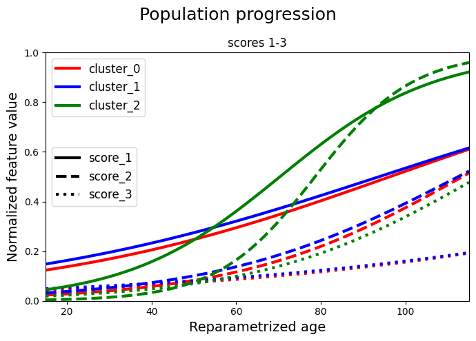
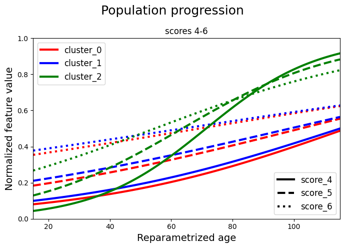
We produce the population progression plots. We separate the model parameters for each cluster and we store them to a dedicated item.

from leaspy.io.outputs import IndividualParameters

parameters = model.parameters
number_of_sources = 2

# cluster 0
mean_xi = parameters["xi_mean"].numpy()[0]
mean_tau = parameters["tau_mean"].numpy()[0]
mean_source = parameters["sources_mean"].numpy()[0, 0].tolist()
mean_sources = [mean_source] * number_of_sources

parameters_0 = {"xi": mean_xi, "tau": mean_tau, "sources": mean_sources}

ip_0 = IndividualParameters()
ip_0.add_individual_parameters("average", parameters_0)

# cluster 1
mean_xi = parameters["xi_mean"].numpy()[1]
mean_tau = parameters["tau_mean"].numpy()[1]
mean_source = parameters["sources_mean"].numpy()[0, 1].tolist()
mean_sources = [mean_source] * number_of_sources

parameters_1 = {"xi": mean_xi, "tau": mean_tau, "sources": mean_sources}

ip_1 = IndividualParameters()
ip_1.add_individual_parameters("average", parameters_1)

# cluster 2
mean_xi = parameters["xi_mean"].numpy()[2]
mean_tau = parameters["tau_mean"].numpy()[2]
mean_source = parameters["sources_mean"].numpy()[0, 2].tolist()
number_of_sources = 2
mean_sources = [mean_source] * number_of_sources

parameters_2 = {"xi": mean_xi, "tau": mean_tau, "sources": mean_sources}

ip_2 = IndividualParameters()
ip_2.add_individual_parameters("average", parameters_2)

We separate the scores and we plot two graphs for clarity. Each cluster is represented with a different colour. Each score is represented with a different linestyle. In the first graph we have the first 3 scores and in the second graph we have the remaining 3 scores. In each graph we plot all the clusters.

from matplotlib.lines import Line2D

timepoints = np.linspace(15, 115, 105)
values_0 = model.estimate({"average": timepoints}, ip_0)
values_1 = model.estimate({"average": timepoints}, ip_1)
values_2 = model.estimate({"average": timepoints}, ip_2)

# A. Scores 1-3

plt.figure(figsize=(7, 5))
plt.ylim(0, 1)
lines = [
    "-",
    "--",
    ":",
]
## cluster 0
for ls, name, val in zip(lines, model.features, values_0["average"][:, 0:3].T):
    plt.plot(timepoints, val, label=f"cluster_0_{name}", c="red", linewidth=3, ls=ls)

## cluster 1
for ls, name, val in zip(lines, model.features, values_1["average"][:, 0:3].T):
    plt.plot(timepoints, val, label=f"cluster_1_{name}", c="blue", linewidth=3, ls=ls)

## cluster 2
for ls, name, val in zip(lines, model.features, values_2["average"][:, 0:3].T):
    plt.plot(timepoints, val, label=f"cluster_2_{name}", c="green", linewidth=3, ls=ls)

## legends
cluster_legend = [
    Line2D([0], [0], color="red", linewidth=3, label="cluster_0"),
    Line2D([0], [0], color="blue", linewidth=3, label="cluster_1"),
    Line2D([0], [0], color="green", linewidth=3, label="cluster_2"),
]
legend1 = plt.legend(handles=cluster_legend, loc="upper left", prop={"size": 12})

color_legend = [
    Line2D([0], [0], linestyle=lines[0], color="black", linewidth=3, label="score_1"),
    Line2D([0], [0], linestyle=lines[1], color="black", linewidth=3, label="score_2"),
    Line2D([0], [0], linestyle=lines[2], color="black", linewidth=3, label="score_3"),
]
legend2 = plt.legend(
    handles=color_legend, loc="center left", title_fontsize=14, prop={"size": 12}
)

plt.gca().add_artist(legend1)

plt.xlim(min(timepoints), max(timepoints))
plt.xlabel("Reparametrized age", fontsize=14)
plt.ylabel("Normalized feature value", fontsize=14)
plt.title("scores 1-3")
plt.suptitle("Population progression", fontsize=18)
plt.tight_layout()
plt.show()

# B. Scores 4-6

plt.figure(figsize=(7, 5))
plt.ylim(0, 1)
lines = [
    "-",
    "--",
    ":",
]
## cluster 0
for ls, name, val in zip(lines, model.features, values_0["average"][:, 3:6].T):
    plt.plot(timepoints, val, label=f"cluster_0_{name}", c="red", linewidth=3, ls=ls)

## cluster 1
for ls, name, val in zip(lines, model.features, values_1["average"][:, 3:6].T):
    plt.plot(timepoints, val, label=f"cluster_1_{name}", c="blue", linewidth=3, ls=ls)

## cluster 2
for ls, name, val in zip(lines, model.features, values_2["average"][:, 3:6].T):
    plt.plot(timepoints, val, label=f"cluster_2_{name}", c="green", linewidth=3, ls=ls)

## legends
cluster_legend = [
    Line2D([0], [0], color="red", linewidth=3, label="cluster_0"),
    Line2D([0], [0], color="blue", linewidth=3, label="cluster_1"),
    Line2D([0], [0], color="green", linewidth=3, label="cluster_2"),
]
legend1 = plt.legend(handles=cluster_legend, loc="upper left", prop={"size": 12})

color_legend = [
    Line2D([0], [0], linestyle=lines[0], color="black", linewidth=3, label="score_4"),
    Line2D([0], [0], linestyle=lines[1], color="black", linewidth=3, label="score_5"),
    Line2D([0], [0], linestyle=lines[2], color="black", linewidth=3, label="score_6"),
]
legend2 = plt.legend(
    handles=color_legend, loc="lower right", title_fontsize=14, prop={"size": 12}
)

plt.gca().add_artist(legend1)

plt.xlim(min(timepoints), max(timepoints))
plt.xlabel("Reparametrized age", fontsize=14)
plt.ylabel("Normalized feature value", fontsize=14)
plt.title("scores 4-6")
plt.suptitle("Population progression", fontsize=18)
plt.tight_layout()
plt.show()

This concludes the Mixture Model example using Leaspy. We can also use these fit models to simulate new data according to the estimated parameters. This can be useful for validating the model, for generating synthetic datasets for further analysis or for generate a trajectory for a new individual given specific parameters. Let’s check this in the next example.