2. Mathematical Background
2.1. Nonlinear mixed effect models
Mixed effects models have become a powerful and widely used statistical tool for analyzing longitudinal, or more specifically repeated measurements, data, especially in the context of biomedical and epidemiological research. These models are particularly suited for studying neurodegenerative and brain diseases where patients are followed over time, and multiple clinical characteristics are measured repeatedly. Moreover these diseases have been known to be heterogenous with subtypes that are often difficult ot characterize.
One of the key strengths of mixed-effects models lies in their ability to capture two types of variability:
Within-subject variability (fixed effects) This reflects systematic influences that affect all patients in similar ways, such as the effect of treatment, demographic factors, or known disease subtypes. Fixed effects represent consistent trends or shifts in the data that apply across the population or across specific groups.
Between-subject variability (random effects) This accounts for differences among individual patients. For example, even if patients share the same diagnosis, their disease progression rates and onset time can vary considerably. By incorporating random effects, the model can capture this heterogeneity, allowing for personalized trajectory estimates at an individual level.
With a mixed effects model, we can estimate the long-term progression of a disease by reconstructing individual patient trajectories over time, even when measurements are irregularly spaced or partially missing. This is crucial for understanding the natural history of a disease, identifying typical progression patterns, and recognizing outliers. Importantly, understanding how a disease evolves over time and quantifying the expected variability between individuals have significant clinical and research implications. Clinically, it supports personalized medicine approaches, tailoring treatment plans based on predicted progression. From a research standpoint, it helps identify factors driving heterogeneity in disease progression, which can inform new hypotheses about disease mechanisms or guide the development of targeted therapies.
Brain and neurodegenerative diseases typically do not progress at a constant rate over time. In this context a non-linear formulation of mixed effects models provides a more realistic and flexible framework for representing the intricate and variable progression patterns. Many biomarkers and clinical symptoms in neurodegeneration follow nonlinear relationships with time or disease stage. Also, nonlinear models can flexibly accommodate this heterogeneity by allowing individual trajectories to differ not only in magnitude but also in shape and timing. For example, some patients may experience a rapid decline early on, while others decline more slowly but for a longer duration.
2.1.1. Parameter estimation
We suppose that the parameters capturing the population and the individual variability, namely fixed and random effects respectively, are latent (\(z\)) follow some prior distributions. The parameters that define these distributions are called namely model parameters (\(\theta\)). We can also include hyperparmeters \(\Pi\) that have known values.
Estimating the parameters of the models can be done through maximisation of the likelihood.
Assuming \(y\) correspond to the observed data, \(z\) the latent parameters, \(\theta\) the model parameters and \(\Pi\) the hyperparameters the likelihood estimated by the model is the following:
\(p(y, z \mid \theta, \Pi)\) can be divided into two different terms: data attachment, which represents how well the model describes the data \(y\), and a prior attachment, which prevents over-fitting:
The prior attachment term can be separated into two terms: two terms for the prior attachment of latent parameters (fixed and random). We end up with the following expression :
A common and well-defined algorithm for the likelihood maximization, proven to converge for non-linear mixed effects models is the MCMC-SAEM.
2.2. Riemannian framework
2.2.1. Disease progression represented as trajectory
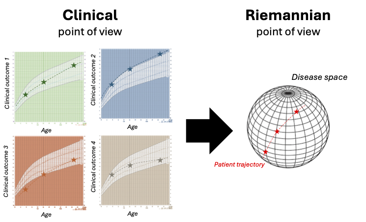
As presented in the figure, the model draws a parallel line between a clinical and a Riemannian point of view of the disease progression.
The idea is to see the variability of the disease progression mapped onto a Riemannian manifold where the longitudinal observations \(y_{i,j,k}\) are aligned in an individual trajectory \(\gamma_i\) that traverses the manifold.
 From clinical to Riemannian point of view (extracted from [27])
From clinical to Riemannian point of view On the left, the progression of four clinical outcomes for one patient is represented depending on the age of the patient. The graph displays the individual progression of one patient on a grid detailing the typical progression of the disease, as it is done in health diaries for BMI curves. This represents how a clinician is used to see the progression of the patient. On the right, progression of the same patient is represented but this time in a disease space (manifold) built thanks to the information extracted from the four clinical outcomes. This represents the Riemannian point of view of the progression of the patient.
2.2.2. Trajectory shape defined by Riemmanian metric
The shape of the disease progression (linear, logistic …) is defined by the choice of the Riemannian metric (\(G(p)\)) applied to the manifold. For instance, the manifold \(\mathbb{R}^n\) equipped with Euclidean metric gives straight lines trajectories and thus straight lines disease progression.
For a K-dimensional dataset, we used the product manifold of a 1-dimensional metric. The disease trajectory is a geodesic if and only if it satisfies a differential equation with the metric, further described in [16] (p.169), or in simple words if it describes the “shortest path” between the observations on the manifold according to the chosen metric. This enables us to obtain the shape of the curve in time from the metric formulation.
Application context: Here, we want to model clinical data such as clinical scores. Such data have a potential floor or ceiling effects [11], thus a logistic curve is often used. The Riemmanian metric \(G(p)\) and the manifold \(M\) that enable to define a logistic progression through time are: \(G(p) = \frac{1}{p^2(1-p)^2}\) an \(M = (0, 1)\).
2.2.3. Disentanglement of parameters with a hierarchical model
2.2.3.1. Population trajectory & Fixed effects:
To separate the average disease progression from the individual progression, a mixed-effects model structure is added to the trajectories.
Any trajectory \(\gamma\) (geodesic) can be defined by the two parameters of its initial condition at a time \(t_0\): the initial position \(\gamma(t_0) = p_0\) and the initial speed \(\dot{\gamma}(t_0) = v_0\).
The average trajectory \(\gamma_0\) is thus parametrized by its initial conditions (\(t_0, v_0, p_0\)) with a shape imposed by the metric.
From there, the individual trajectory \(\gamma_i(t)\) could be defined playing on the three initial conditions.
2.2.3.2. Individual trajectory & Temporal random effects:
If a patient starts to have symptoms of the disease \(\tau_i - t_0\) earlier (later) than the average population, it impacts the initial condition with (\( \tau_i \), \( v_0, p_0\)).
A second option, is that the patient will have a faster (slower) disease progression with a factor \(e^{\xi_i}\). This time, initial conditions are impacted so that (\( t_0, v_0 \), \( e^{\xi_i} \) \(, p_0\)). Note that the two first aspects encompass temporal variability.
From a mathematical point of view these impacts could be seen as a transformation of the age of the patient into a latent disease age, as the effect on the trajectory is restricted to the reparametrisation of the time by the formula \(\psi_i(t) = v_0 e^{\xi_i} (t -\tau_i) + t_0\).
2.2.3.3. Individual trajectory & Spatial random effects
Finally, patients may vary in terms of disease presentation, i.e. from a clinical point of view, meaning that the order of outcome progression might differ between individuals.
From a geometric point of view, this means that the geometric trajectory is not overlapping through the same points. This variability is enabled by manipulating the initial position \(p_0\). It is done thanks to the vectors \( w_k \) named space-shifts in the tangent space of the manifold that modified the trajectory in the sense of the Exp-parallelisation to assure the identifiability.
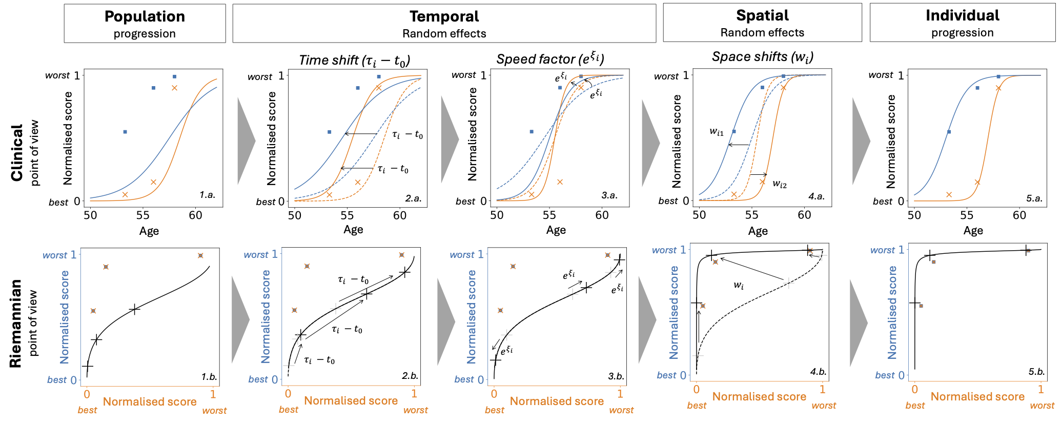 Temporal and spatial random effects: from population to individual progression (extracted from [27])
This figure presents from two points of view (clinical and Riemannian) how the three types of random effects (two temporal and one spatial) enable to modify the population average progression to calibrate the patient observations. Clinical: Two normalised clinical scores (blue and orange) (0: the healthiest value, +1: the maximum pathological change) depending on the age of the patients. The scatter represents the real observed values for one patient at different visits. Riemannian: The same two normalised scores are represented but this time depending on each other. The scatter represents the same real observed values as in the clinical version. The black cross on the curve corresponds to what is modelled at the visit ages of the patient.
Temporal and spatial random effects: from population to individual progression (extracted from [27])
This figure presents from two points of view (clinical and Riemannian) how the three types of random effects (two temporal and one spatial) enable to modify the population average progression to calibrate the patient observations. Clinical: Two normalised clinical scores (blue and orange) (0: the healthiest value, +1: the maximum pathological change) depending on the age of the patients. The scatter represents the real observed values for one patient at different visits. Riemannian: The same two normalised scores are represented but this time depending on each other. The scatter represents the same real observed values as in the clinical version. The black cross on the curve corresponds to what is modelled at the visit ages of the patient.
Population progression (1.a., 1.b.): Population average trajectory compared to the observed values of the patient.
Time Shift (2.a., 2.b.): The progression starts earlier due to the individual estimated reference time, Clinical graph: the curves are shifted on the left, Riemannian graph: black crosses are shifted on the right following the trajectory (for the same age the patient is more advanced).
Speed factor (3.a., 3.b.): The progression speed increases, Clinical graph: the curves become steeper, Riemannian graph: black crosses get further from each other on the trajectory (for the same time of follow-up a wider portion of the trajectory is observed).
Space Shift (4.a., 4.b.): the blue curves progress before the orange curve, Clinical graph: the curves are shifted in opposite directions, Riemannian graph: most of the blue (resp. orange) score value is observed for an orange (resp. blue) value of 0 (resp. 1)
Individual progression (5.a., 5.b.): The modelled curves fit the observations, Riemannian graph: the black crosses are close to the observed values.
2.3. References
Paul H. Gordon, Bin Cheng, Francois Salachas, Pierre-Francois Pradat, Gaelle Bruneteau, Philippe Corcia, Lucette Lacomblez, and Vincent Meininger. Progression in als is not linear but is curvilinear. Journal of Neurology, 257(10):1713–1717, October 2010. doi:10.1007/s00415-010-5609-1.
Igor Koval. Learning Multimodal Digital Models of Disease Progression from Longitudinal Data : Methods & Algorithms for the Description, Prediction and Simulation of Alzheimer’s Disease Progression. phdthesis, Institut Polytechnique de Paris, January 2020. URL: https://theses.hal.science/tel-02524279 (visited on 2025-05-07).
Juliette Ortholand. Joint modelling of events and repeated observations : an application to the progression of Amyotrophic Lateral Sclerosis. phdthesis, Sorbonne Université, September 2024. URL: https://theses.hal.science/tel-04770912 (visited on 2025-05-07).