5. Models Evaluation
5.1. Convergence diagnosis
When using leaspy, you have to choose the number of iterations to estimate the model and hopefully to reach convergence of the MCMC-SAEM algorithm used. A famous way to monitor it is by running several MC chains with various random seeds and compute the statistic of Gelman-Rubin[10], denoted \(\hat{R}\). The \(\hat{R}\) measures the ratio of the within-chain variance to the between-chain variance. If the chain has converged to the same stationary distribution, these two variances should be roughly equal[40].
where \(W\) is the within-chain variance and \(\hat{V}\) is the posterior variance estimate for the pooled rank-traces.
This could be computed thanks to the package arviz with the function rhat.
5.2. Fit metrics
Leaspy stores three negative log likelihood (nll) values in the fit_metrics of the model’s json file:
nll_attach: \(-\log p(y \mid z, \theta, \Pi)\), where \(y\) are the observations, \(z\) the latent parameters, \(\theta\) the model parameters, and \(\Pi\) the hyperparameters. It corresponds to the nll attached to the data.nll_regul_ind_sum: \(-\log p(z_{\text{re}} \mid z_{\text{fe}}, \theta, \Pi)\), where \(z_{\text{re}}\) denotes the latent random effects and \(z_{\text{fe}}\) the latent fixed effects. It corresponds to the nll from the random effects.nll_tot: \(-\log p(y, z, \theta \mid \Pi)\). It corresponds to the total nll: nll_attach, nll_regul_ind_sum and the nll linked to the fixed effects \(-\log p(z_{\text{fe}} \mid \theta, \Pi)\), that is not reported directly in the json file.
The last conditional nll can be used for computing fit metrics.
5.2.1. Bayesian Approach
5.2.1.1. WAIC
WAIC (Watanabe – Akaike information criterion), defined by Watanabe in 2010 [42], is a metric permitting comparing different Bayesian models. Lower values of WAIC correspond to better performance of the model.
For example, the version by Vehtari, Gelman, and Gabry (2017) [39] can be used in the Leaspy framework, with β = 1 and multiplied by -2 to be on the deviance scale. To compute it, the probability of observation given the parameters should be computed for each iteration. Two versions can be computed using the conditional or the marginal likelihood.
The marginal likelihood is more robust [24], but it is harder to compute as the integral must be estimated. It is usually estimated using Laplace’s approximation, which corresponds to a Taylor expansion [7].
Where \(p(y_i | \hat{\theta}_i)\) is the probability of the observation given the estimated parameters \(\hat{\theta}_i\), and \(n\) is the number of data points.
5.2.2. Frequentist Approach
5.2.2.1. AIC
AIC (Akaike Information Criterion) is a robust metric for model selection that quantifies the balance between goodness-of-fit and model complexity. It has a penalty term for the number of parameters in the model, thus penalizing more complex models with unnecessary features. Lower AIC values indicate a better model [1].
# Get the negative log-likelihood
nll = model.state['nll_attach']

# Compute the number of free parameters
free_parameters_total = (
    3 + 2 * model.dimension + (model.dimension - 1) * (model.source_dimension)
)

penalty = 2 * free_parameters_total

aic = penalty + 2 * nll
print(f"AIC: {aic}")

AIC: -17236.7421875
5.2.2.2. BIC
BIC (Bayesian Information Criterion) is similar to the AIC metric, but applies a stronger penalty that depends on the number of observations [37]. It tends to favor simpler models more strongly than AIC.
# Get the negative log-likelihood
nll = model.state['nll_attach']

# Compute the number of free parameters
free_parameters_total = (
    3 + 2 * model.dimension + (model.dimension - 1) * (model.source_dimension)
)

n_observations = data.n_visits
penalty = free_parameters_total * np.log(n_observations)

bic = penalty + 2 * nll
print(f"BIC: {bic}")

BIC: -12671.0820312
5.3. Prediction metrics
These metrics could be computed either on predictions or in reconstructions. Note that all this could be stratified by the different groups you have in your dataset. You might want these metrics to be independent from it.
5.3.1. Repeated Measures
This section describes the main metrics used to evaluate the quality of predictions from the Leaspy non-linear mixed-effects model.
5.3.1.1. Mean Absolute Error (MAE)
MAE is more robust to outliers than MSE, and provides a straightforward sense of typical prediction error.
For more information, please see sklearn.metrics.
from sklearn.metrics import mean_absolute_error

# Keep the TIME we want to predict at
alzheimer_df_to_pred = alzheimer_df.groupby('ID').tail(1)
# Predict using estimate
reconstruction = model.estimate(alzheimer_df_to_pred.index, individual_parameters)
df_pred = reconstruction.add_suffix('_model1')
# Compute the MAE
mae = mean_absolute_error(alzheimer_df_to_pred["MMSE"], df_pred["MMSE_model1"])
print(f"Mean Absolute Error: {mae}")

Mean Absolute Error: 0.050412963298149406
5.3.1.2. Mean Square Error (MSE)
MSE penalizes larger errors more heavily than MAE, making it more sensitive to outliers [43][5].
For more information, please see sklearn.metrics.
from sklearn.metrics import mean_squared_error

# Keep the TIME we want to predict at
alzheimer_df_to_pred = alzheimer_df.groupby('ID').tail(1)
# Predict using estimate
reconstruction = model.estimate(alzheimer_df_to_pred.index, individual_parameters)
df_pred = reconstruction.add_suffix('_model1')
# Compute the MSE
mse = mean_squared_error(alzheimer_df_to_pred["MMSE"], df_pred["MMSE_model1"])
print(f"Mean Squared Error: {mse}")

Mean Squared Error: 0.0041833904503857655
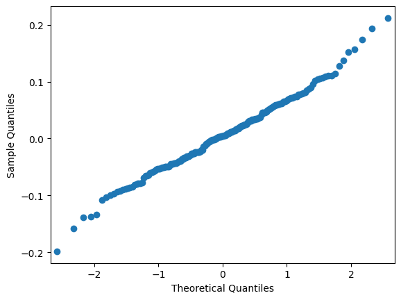
5.3.1.3. Residual Q-Q Plot
A graphical tool to assess whether residuals follow a normal distribution, which is an assumption in many mixed-effects models [9].
For more information, please see statsmodels.api.
import statsmodels.api as sm
from matplotlib import pyplot as plt

# Compute the residuals
res = alzheimer_df_to_pred["MMSE"] - df_pred["MMSE_model1"]
fig = sm.qqplot(res)
plt.show()
5.3.1.4. Coefficient of Determination (R²)
R² indicates how well the model explains the variance in the observed data. Higher values (closer to 1) suggest better performance.
In mixed-effects models, multiple R² variants exist (e.g., marginal vs. conditional R²) to account for fixed and random effects [26].
For more information, please see sklearn.metrics.
from sklearn.metrics import r2_score
r2 = r2_score(alzheimer_df_to_pred["MMSE"], df_pred["MMSE_model1"])
print(f"R² Score: {r2}")

R² Score: 0.9442675319358963
5.3.2. Events
For the joint model, it is useful to have prediction metrics on survival as well:
5.3.2.1. Integrated Brier Score (IBS)
The Integrated Brier Score (IBS) is a robust metric used to evaluate the predictive accuracy of survival models. In survival analysis, IBS quantifies how well a model predicts the timing of events by integrating the Brier Score, a measure of prediction error for probabilistic outcomes, across all observed time points. It compares the model’s predicted survival probabilities against actual observed outcomes, penalizing discrepancies between predictions and reality. IBS accounts for censored data, ensuring reliability in real-world datasets where not all events are fully observed. IBS describes how closely predictions match reality. A low IBS indicates superior predictive performance, as it reflects smaller cumulative errors over time [12].
For more information, please see scikit-survival.
5.3.2.2. Cumulative Dynamic AUC
Cumulative AUC (or time-dependent AUC) evaluates the model’s ability to discriminate between subjects who experience an event by a specific time and those who do not, based on their predicted risk scores. It focuses on ranking accuracy, ensuring high-risk subjects receive higher predicted probabilities than low-risk ones at each time point. Cumulative AUC describes how well risks are ordered. A high cumulative AUC means a strong discriminatory ability [] [13] [19].
For more information, please see scikit-survival.
5.3.2.3. Avoid using C-index
The C-index or Concordance index, similarly to the cumulative AUC, is a metric assessing the discriminatory ability of a survival model. However, this metric is criticized because it is a global metric that averages performance over the entire study period, hiding time-specific weaknesses [4]. It also depends on the censoring distribution. Therefore, it is more convenient to use time-dependent AUC and the Brier Score presented above.
5.4. References
H. Akaike. A new look at the statistical model identification. IEEE Transactions on Automatic Control, 19(6):716–723, 1974. doi:10.1109/TAC.1974.1100705.
P. Blanche, M. W. Kattan, and T. A. Gerds. The c-index is not proper for the evaluation of predicted risks for specific years. Statistics in Medicine, 38(14):2682–2697, 2019. doi:10.1002/sim.8042.
T. Chai and R. R. Draxler. Root mean square error (rmse) or mean absolute error (mae)? – arguments against avoiding rmse in the literature. Geoscientific Model Development, 7(3):1247–1254, 2014. doi:10.5194/gmd-7-1247-2014.
P. Daxberger and et al. Laplace approximation for bayesian inference. In Proceedings of NeurIPS, 1–8. 2021. URL: https://proceedings.neurips.cc/paper/2021/hash/a7c9585703d275249f30a088cebba0ad-Abstract.html.
J. Fox. Applied Regression Analysis and Generalized Linear Models. Sage Publications, 2015.
Andrew Gelman and Donald B. Rubin. Inference from iterative simulation using multiple sequences. Statistical Science, 7(4):457–472, 1992.
E. Graf, C. Schmoor, W. Sauerbrei, and M. Schumacher. Assessment and comparison of prognostic classification schemes for survival data. Statistical Medicine, 18(17-18):2529–2545, 1999. doi:10.1002/(sici)1097-0258(19990915/30)18:17/18<2529::aid-sim274>3.0.co;2-5.
H. Hung and C. T. Chiang. Estimation methods for time-dependent auc models with survival data. Canadian Journal of Statistics, 38(1):8–26, 2010.
J. Lambert and S. Chevret. Summary measure of discrimination in survival models based on cumulative/dynamic time-dependent roc curves. Statistical Methods in Medical Research, 2014.
R. Millar. Bayesian model checking. Statistical Modelling, 18(4):417–435, 2018.
S. Nakagawa and H. Schielzeth. A general and simple method for obtaining r2 from generalized linear mixed-effects models. Methods in Ecology and Evolution, 3(2):129–142, 2012. doi:10.1111/j.2041-210X.2012.00261.x.
G. Schwarz. Estimating the dimension of a model. Annals of Statistics, 6(2):461–464, 1978. doi:10.1214/aos/1176344136.
A. Vehtari, A. Gelman, and J. Gabry. Practical bayesian model evaluation using leave-one-out cross-validation and waic. Statistics and Computing, 27(5):1413–1432, 2017. URL: https://arxiv.org/pdf/1507.04544.
Aki Vehtari, Andrew Gelman, Daniel Simpson, Bob Carpenter, and Paul-Christian Bürkner. Rank-normalization, folding, and localization: an improved rˆ for assessing convergence of mcmc (with discussion). Bayesian Analysis, June 2021. URL: http://dx.doi.org/10.1214/20-BA1221, doi:10.1214/20-ba1221.
S. Watanabe. Asymptotic equivalence of the bayesian and widely applicable information criteria. Journal of Machine Learning Research, 11:3571–3594, 2010. URL: https://www.jmlr.org/papers/volume11/watanabe10a/watanabe10a.pdf.
C. J. Willmott and K. Matsuura. Advantages of the mean absolute error (mae) over the root mean square error (rmse). Climate Research, 30(1):79–82, 2005.